How does one plot the torque and horsepower curves for a 1999 Miata ? In this blog post, we explain how to do that using some dynamometer or dyno data from someone else’s 99 Miata. I have not taken my Miata to a dyno yet but this should be enough for an example for your car or for any other car, as long as you have the data.
The rest of the data specific to a factory 1999 MX-5 Miata (base trim and 10th Anniversary Edition) can be taken from here, which I provide as miata99_data_power.csv for download and also shown in the table below.
For all the engineering or physics related calculations in this blog, I will be using Octave, a free and open source tool for scientific calculations. If you have used MATLAB or have never used anything except Microsoft Excel, Octave should be relatively easy to convert the physics equations into quick running code, which I will explain as we go along.
| Engine RPM | Wheel Torque (Nm) | Wheel Torque (lb-ft) | Wheel Horsepower (kW) | Wheel horsepower (PS) or (bhp) or metric hp | Wheel Horsepower (hp) mechanical |
|---|---|---|---|---|---|
| 1000 | 72.3 | 53.3 | 7.6 | 10.3 | 10.1 |
| 1100 | 82.1 | 60.5 | 9.5 | 12.9 | 12.7 |
| 1200 | 90.4 | 66.7 | 11.4 | 15.5 | 15.2 |
| 1300 | 97.3 | 71.8 | 13.2 | 18 | 17.8 |
| 1400 | 103.3 | 76.2 | 15.1 | 20.6 | 20.3 |
| 1500 | 108.4 | 79.9 | 17 | 23.2 | 22.8 |
| 1600 | 112.9 | 83.3 | 18.9 | 25.7 | 25.3 |
| 1700 | 116.9 | 86.2 | 20.8 | 28.3 | 27.9 |
| 1800 | 120.5 | 88.9 | 22.7 | 30.9 | 30.4 |
| 1900 | 123.6 | 91.2 | 24.6 | 33.4 | 33 |
| 2000 | 126.5 | 93.3 | 26.5 | 36 | 35.5 |
| 2100 | 129.1 | 95.2 | 28.4 | 38.6 | 38 |
| 2200 | 131.4 | 96.9 | 30.3 | 41.2 | 40.6 |
| 2300 | 133.6 | 98.5 | 32.2 | 43.8 | 43.1 |
| 2400 | 135.5 | 99.9 | 34.1 | 46.3 | 45.6 |
| 2500 | 137.3 | 101.3 | 35.9 | 48.9 | 48.2 |
| 2600 | 139 | 102.5 | 37.8 | 51.5 | 50.7 |
| 2700 | 140.6 | 103.7 | 39.8 | 54.1 | 53.3 |
| 2800 | 142 | 104.7 | 41.6 | 56.6 | 55.8 |
| 2900 | 143.3 | 105.7 | 43.5 | 59.2 | 58.3 |
| 3000 | 144.6 | 106.6 | 45.4 | 61.8 | 60.9 |
| 3100 | 145.7 | 107.4 | 47.3 | 64.3 | 63.4 |
| 3200 | 146.8 | 108.3 | 49.2 | 66.9 | 65.9 |
| 3300 | 147.9 | 109.1 | 51.1 | 69.5 | 68.5 |
| 3400 | 148.8 | 109.7 | 53 | 72.1 | 71 |
| 3500 | 149.7 | 110.4 | 54.9 | 74.6 | 73.5 |
| 3600 | 150.6 | 111.1 | 56.8 | 77.2 | 76.1 |
| 3700 | 151.4 | 111.7 | 58.7 | 79.8 | 78.6 |
| 3800 | 152.2 | 112.2 | 60.6 | 82.4 | 81.2 |
| 3900 | 152.9 | 112.8 | 62.4 | 84.9 | 83.7 |
| 4000 | 153.6 | 113.3 | 64.3 | 87.5 | 86.2 |
| 4100 | 154.3 | 113.8 | 66.3 | 90.1 | 88.8 |
| 4200 | 154.9 | 114.2 | 68.1 | 92.7 | 91.3 |
| 4300 | 155.5 | 114.7 | 70 | 95.2 | 93.8 |
| 4400 | 156.1 | 115.1 | 71.9 | 97.8 | 96.4 |
| 4500 | 156.6 | 115.5 | 73.8 | 100.4 | 98.9 |
| 4600 | 157.1 | 115.9 | 75.7 | 102.9 | 101.4 |
| 4700 | 157.6 | 116.2 | 77.6 | 105.5 | 103.9 |
| 4800 | 158.1 | 116.6 | 79.5 | 108.1 | 106.5 |
| 4900 | 158.6 | 117 | 81.4 | 110.7 | 109.1 |
| 5000 | 159 | 117.3 | 83.3 | 113.2 | 111.6 |
| 5100 | 159.5 | 117.6 | 85.2 | 115.9 | 114.2 |
| 5200 | 159.9 | 117.9 | 87.1 | 118.4 | 116.7 |
| 5300 | 160.3 | 118.2 | 89 | 121 | 119.2 |
| 5400 | 160.6 | 118.4 | 90.8 | 123.5 | 121.7 |
| 5500 | 161 | 118.7 | 92.7 | 126.1 | 124.3 |
| 5600 | 160.9 | 118.7 | 94.4 | 128.3 | 126.4 |
| 5700 | 160.7 | 118.5 | 95.9 | 130.5 | 128.5 |
| 5800 | 160.3 | 118.2 | 97.4 | 132.4 | 130.5 |
| 5900 | 159.8 | 117.8 | 98.7 | 134.3 | 132.3 |
| 6000 | 159.1 | 117.3 | 100 | 136 | 134 |
| 6100 | 158.3 | 116.7 | 101.1 | 137.5 | 135.5 |
| 6200 | 157.3 | 116 | 102.1 | 138.9 | 136.9 |
| 6300 | 156.2 | 115.2 | 103.1 | 140.2 | 138.1 |
| 6400 | 154.9 | 114.2 | 103.8 | 141.2 | 139.1 |
| 6500 | 153.5 | 113.2 | 104.5 | 142.1 | 140 |
| 6600 | 150.6 | 111.1 | 104.1 | 141.6 | 139.5 |
| 6700 | 146.6 | 108.1 | 102.9 | 139.9 | 137.8 |
| 6800 | 141.5 | 104.4 | 100.8 | 137 | 135 |
| 6900 | 135.4 | 99.9 | 97.8 | 133.1 | 131.1 |
| 7000 | 128.3 | 94.6 | 94.1 | 127.9 | 126 |
Comments in Octave start with the # character, so in the code below I describe each line for those who are reading this and are unfamiliar with programming.
The below code plots the above table data (also in CSV) in both metric units and imperial units.
## load the data from the CSV file
data = csvread("miata99_data_power.csv")

## clear the figure window
clf

## plot Torque in Nm in the color red and Wheel Horsepower in kW in color green
## set the x-axis, y-axes labels, the title and save the plot to a file
ax = plotyy(data(2:end, 1), data(2:end, 2), data(2:end, 1), data(2:end, 4))
xlabel("RPM")
ylabel(ax(1), "Torque (Nm)")
ylabel(ax(2), "Horsepower (kW)")
title("Torque - Horsepower Curve (metric units)")
grid on
print("torquehp_metric.png")

## plot Torque in lb-ft in the color red and Wheel Horsepower in hp in color green
## set the x-axis and y-axis label and save the plot to a file
clf
ax = plotyy(data(2:end, 1), data(2:end, 3), data(2:end, 1), data(2:end, 6))
xlabel("RPM")
ylabel(ax(1), "Torque (lb-ft)")
ylabel(ax(2), "Horsepower (hp)")
title("Torque - Horsepower Curve (imperial units)")
grid on
print("torquehp_imperial.png")
The saved plots are presented below.
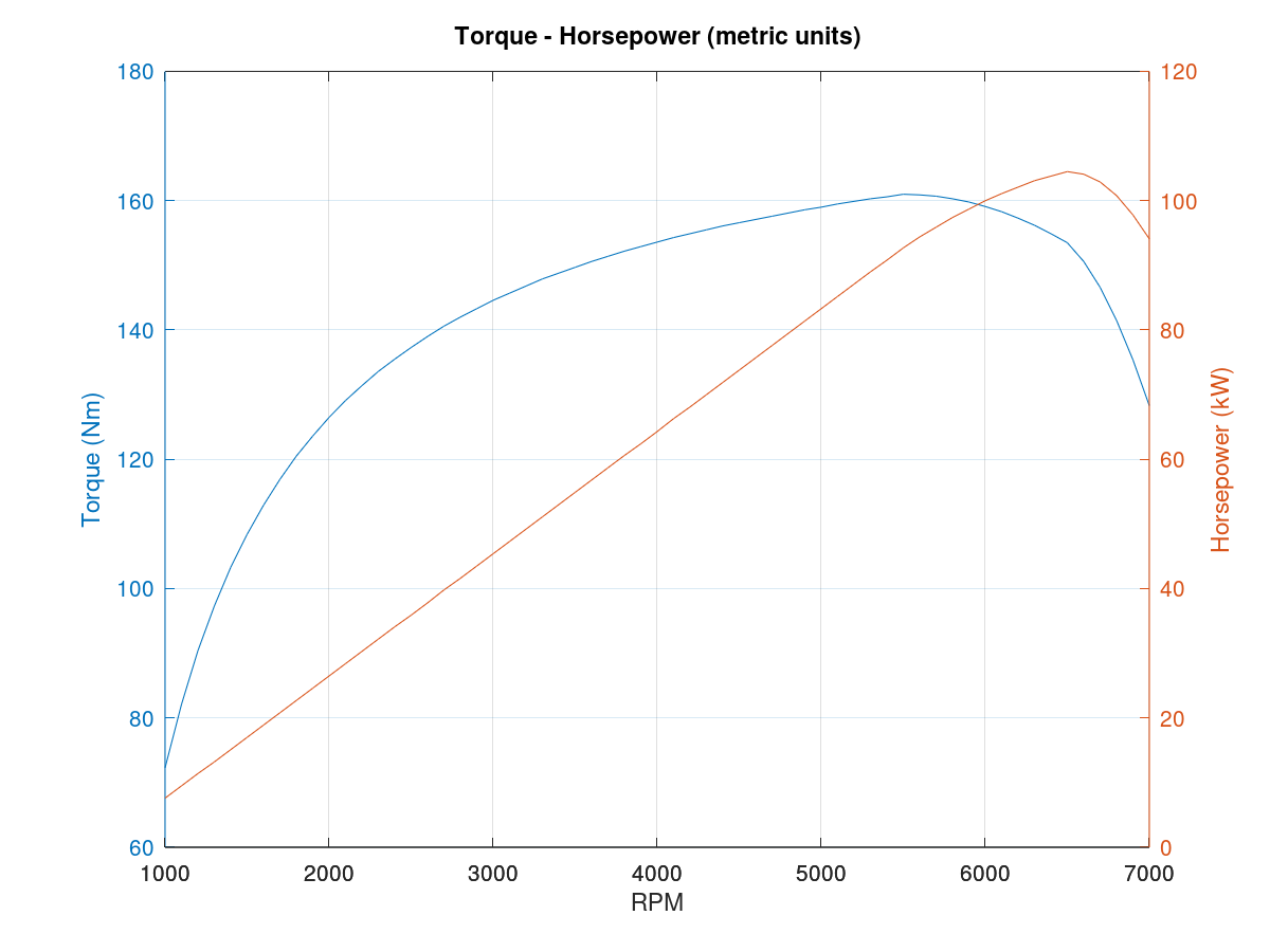 Figure 1. Plot of Torque-horsepower curve in metric units
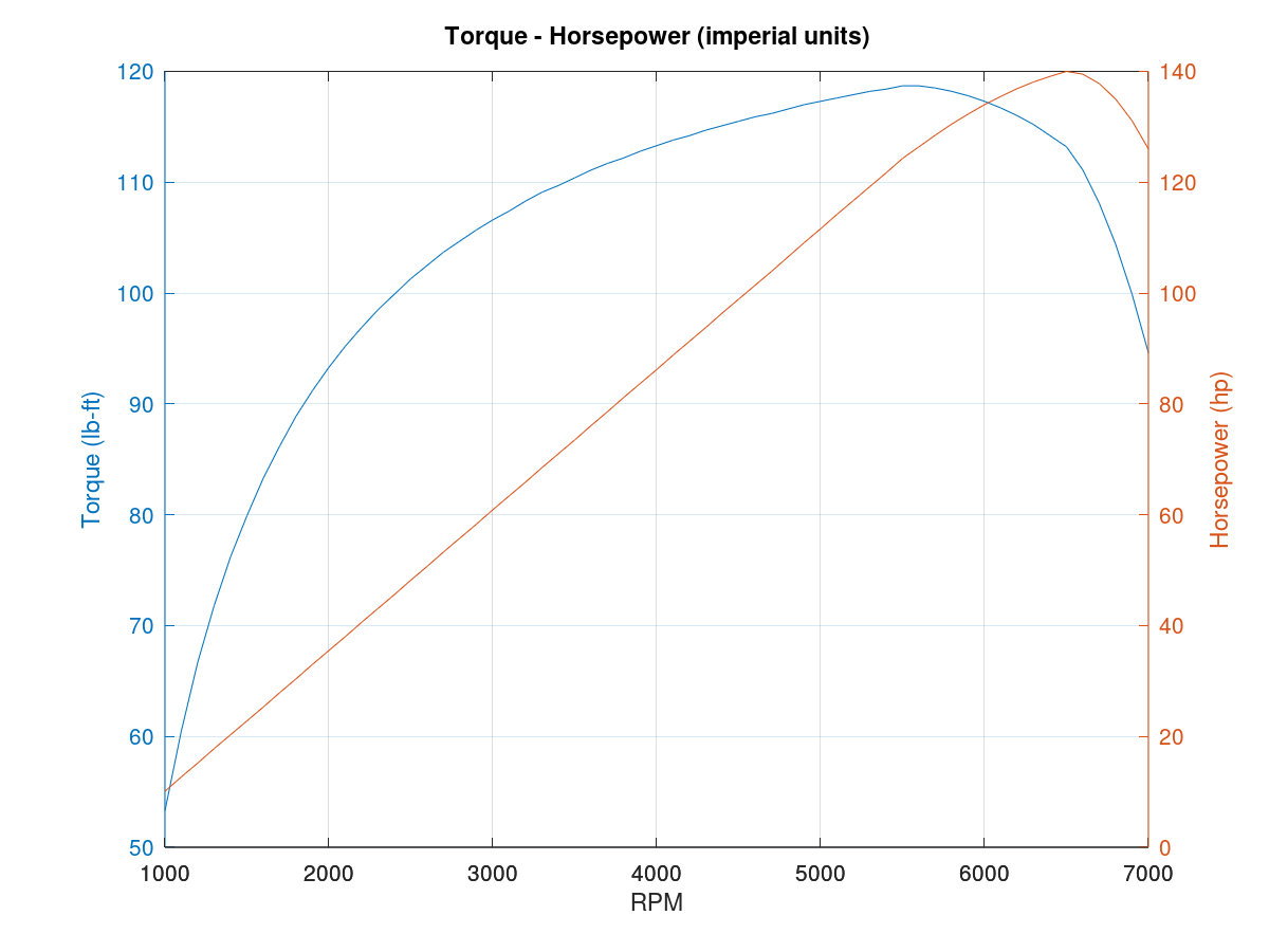 Figure 2. Plot of Torque-horsepower curve in imperial units
As you may notice in both the plots above, regardless of the units the plots look alike. The torque curve (in blue) shows that the wheel torque rises as the RPM increases faster below 3000 RPM, after which the rise in torque is slower until it reaches 5500 RPM, after which any increase in RPM leads to a decrease in torque. Manufacturers, such as Mazda, generally quote the maximum torque values at this RPM point of 5500 RPM as it is the case for the NB Miata.
Similarly the horsepower increases steadily until 6500 RPM is reached after which it starts dropping. In many other vehicles the RPM levels are going to be lower, but in the Miata the maximum horsepower is attained at very high RPMs. This suggests that the driver can accelerate in the same gear to 5500 RPM, as acceleration is related to torque, to get maximum torque at the wheels. However, the maximum horsepower will be achieved at a higher RPM and the best compromise is to try to attain the intersection point of the two curves which is between 6000 and 6100 RPM.
As an autocross driver is most likely going to be driving in second gear, it makes sense to try to push the car to at least 5500 RPM to be as fast as possible. That is something I want to try out in my next autocross event.